This article presents a systematic test and analysis of matrix multiplication performance across various hardware and software implementations. Based on a high-performance computing node equipped with multi-core CPUs and multiple GPUs, I will start from the most basic algorithmic implementation and progressively examine performance differences across different layers: compiler optimization, specialized computing libraries, GPU parallel computing, and multi-device distributed computing. By comparing detailed performance data, we reveal how hardware characteristics and software implementations collectively influence final computational efficiency.
Barkla2 HPC
The hardware configuration of the computing node used in this test is as follows. The Central Processing Units (CPUs) consist of two Intel Xeon Gold 5218 processors, totaling 32 physical cores, with a base frequency of 2.30 GHz and Turbo Boost support. These CPUs support the AVX-512 vector instruction set and FMA (Fused Multiply-Add) operations, which are crucial for accelerating floating-point matrix operations. The memory system includes a three-level cache: each core has independent L1 and L2 caches (32KB and 1MB respectively), while all cores share a 23MB L3 cache. The system utilizes a NUMA (Non-Uniform Memory Access) architecture with two NUMA nodes; remote memory access latency is significantly higher than local memory access.
The Graphics Processing Units (GPUs) include four NVIDIA Tesla V100-PCIE-16GB cards. Each GPU features 5120 CUDA cores and 80 Streaming Multiprocessors (SMs). Notably, it includes 640 Tensor Cores, which provide extremely high throughput for half-precision (FP16) matrix operations. Each GPU is equipped with 16GB of HBM2 memory, offering approximately 900GB/s of bandwidth.
The interconnect topology between devices significantly impacts multi-GPU performance. Between GPU0 and GPU1, as well as GPU2 and GPU3, high-speed NVLink interconnects (labeled as NODE) are used, each associated with one of the two NUMA nodes. In contrast, GPU pairs located on different nodes (e.g., GPU0 and GPU2) are connected via slower PCIe and UPI paths (labeled as SYS). This architecture implies that in distributed computing, algorithms should minimize cross-node communication to optimize performance.
Next is the benchmark implementation using C++ and CUDA. We start with the most basic implementation, gradually adding optimizations—first on the CPU, then transitioning to the GPU. This section demonstrates how hardware features translate into actual performance gains.
The methodology used for testing is critical. The benchmark pre-allocates a random matrix pool. Each timed iteration randomly selects a pair of matrices from the pool for calculation. This design helps prevent data from staying excessively in high-speed cache due to repeated use, thereby measuring computational throughput that is more representative of real-world scenarios.
Naive Algorithm
We first analyze the most basic matrix multiplication implementation: the triple-nested loop. This is the most direct translation of the algorithm.
The core code example is as follows:
void cpu_naive_sgemm(int N, const float* A, const float* B, float* C) {
    for (int i = 0; i < N; ++i) {
        for (int k = 0; k < N; ++k) {
            float temp = A[i * N + k];
            for (int j = 0; j < N; ++j) {
                C[i * N + j] += temp * B[k * N + j];
            }
        }
    }
}
The code adopts an (i, k, j) loop order. In the innermost j loop, the program accesses one row of matrix C and one row of matrix B sequentially. This memory access pattern is efficient as it aligns with how CPU caches prefetch contiguous data blocks (cache lines) from memory. Storing A[i * N + k] in a temporary variable temp helps the compiler keep it in a register, further increasing access speed.
However, this implementation has fundamental limitations. First, it is entirely sequential, utilizing only a single CPU core. Second, it does not explicitly leverage vector instruction units like AVX-512. While advanced compilers may attempt auto-vectorization under aggressive optimization, the results are usually inferior to manual optimization.
Benchmark results reflect these constraints. When the matrix size , the average execution time is approximately 214 microseconds, with performance around 20 GFLOPS. When increases to 1024, the execution time jumps to 185 milliseconds, and performance drops to about 11.6 GFLOPS. This performance degradation is a typical manifestation of the memory hierarchy: smaller matrices can mostly reside in the cache, while larger matrices (e.g., a 1024x1024 matrix occupying about 12MB) exceed cache capacity, forcing CPU cores to wait frequently for data from main memory. Consequently, testing skipped larger sizes of and 4096.
This naive implementation establishes a performance baseline, demonstrating the limits of a single-core CPU when facing memory access bottlenecks.
OpenMP
The primary bottleneck of the naive implementation is the use of only one CPU core. To utilize the other cores on the machine, we use OpenMP for parallelization. OpenMP uses compiler directives to guide the parallel execution of loops.
The code modification is minimal, primarily adding a single line before the outer loop:
void cpu_omp_sgemm(int N, const float* A, const float* B, float* C) {
    #pragma omp parallel for
    for (int i = 0; i < N; ++i) {
        // ... inner loops remain unchanged
    }
}
The #pragma omp parallel for directive creates a pool of threads (set to 32, the number of cores, via the OMP_NUM_THREADS environment variable) and distributes iterations of the following i loop among them. Since each thread is responsible for calculating different rows of the output matrix C, no data races occur.
The build script uses find_package(OpenMP REQUIRED) to configure the compilation environment, adding necessary flags (such as -fopenmp for GCC).
Performance improvement is significant. At , the average execution time decreased from 214 microseconds to 15.8 microseconds, a speedup of about 13.5x. At , time decreased from 185 milliseconds to 5.6 milliseconds, a speedup of roughly 33x, close to the ideal scaling for 32 cores. This indicates that for large-scale matrix multiplication, the computation can be effectively parallelized across multiple cores with relatively low thread management overhead.
A key code fix is worth noting: an earlier version attempted to use the collapse(2) clause to parallelize the two outer loops, but this caused multiple threads to write to the same row of matrix C simultaneously, triggering data races. The fixed version parallelizes only the outermost i loop, ensuring each thread writes to independent rows, thus guaranteeing correctness.
The OpenMP version significantly boosts performance with minimal code changes, fully utilizing multi-core CPU power. However, it still relies on the compiler for vectorization of the inner loops.
OpenMP+SIMD
While OpenMP achieves multi-core parallelism, each core still primarily executes scalar operations. To further enhance performance, we must leverage SIMD (Single Instruction, Multiple Data) capabilities. The Xeon Gold 5218 CPU supports the AVX-512 instruction set, which can process 16 single-precision floats simultaneously. The AVX512_OMP benchmark uses AVX-512 intrinsics to explicitly control vectorization.
The code structure is similar to the OpenMP version, with the outer loop parallelized by OpenMP. The main difference is the innermost j loop, rewritten using AVX-512 instructions:
void cpu_avx512_sgemm(int N, const float* A, const float* B, float* C) {
    #pragma omp parallel for
    for (int i = 0; i < N; ++i) {
        for (int k = 0; k < N; ++k) {
            __m512 a_val = _mm512_set1_ps(A[i * N + k]);
            for (int j = 0; j < N; j += 16) {
                __m512 b_val = _mm512_loadu_ps(&B[k * N + j]);
                __m512 c_val = _mm512_loadu_ps(&C[i * N + j]);
                c_val = _mm512_fmadd_ps(a_val, b_val, c_val);
                _mm512_storeu_ps(&C[i * N + j], c_val);
            }
        }
    }
}
The logic is as follows:
__m512is a 512-bit vector data type containing 16 floats._mm512_set1_psbroadcasts a scalar value to all 16 positions in a vector.- The inner loop increment is 16, as each AVX-512 instruction handles 16 floats.
_mm512_loadu_psloads 16 contiguous floats from memory into a vector register (uallows unaligned addresses)._mm512_fmadd_psperforms the fused multiply-add operation , the core of matrix multiplication._mm512_storeu_psstores the result vector back to memory.
Performance results show that at , the OpenMP version took about 5.6 ms, and the AVX-512 version also took roughly 5.6 ms—virtually no difference. This indicates that when using -Ofast -march=native flags, the modern GCC compiler is already capable of auto-vectorizing the inner loop of the OpenMP version, generating code as efficient as manual AVX-512 intrinsics.
This outcome demonstrates that for well-structured loops, compilers can perform effective auto-vectorization. Manual intrinsics did not yield significant extra performance here; their primary value was verifying that compiler optimization had already reached the algorithmic limit on this CPU.
OpenBLAS
In actual high-performance computing, one rarely implements standard matrix multiplication from scratch but rather uses highly optimized libraries. BLAS (Basic Linear Algebra Subprograms) defines the standard interface for such computations, and OpenBLAS is a widely used open-source implementation.
The OpenBLAS benchmark replaces our previous triple loop with a single function call:
cblas_sgemm(CblasRowMajor, CblasNoTrans, CblasNoTrans, N, N, N,
            1.0f, A, N, B, N, 0.0f, C, N);
Behind this single line are kernels meticulously optimized for various CPU architectures, often written in assembly and employing advanced optimization techniques:
- Cache Blocking: Breaking matrices into blocks that fit into CPU cache levels (L1, L2, L3) to reduce data movement between memory and cache.
- Register Blocking: Further subdivision to maximize data usage within CPU registers, the fastest storage units.
- Prefetching: Using specific instructions to load data from memory to cache in advance, hiding memory latency.
- Loop Unrolling: Expanding inner loops to reduce control overhead and provide more instruction-level parallelism for the CPU’s out-of-order execution engine.
Performance results clearly demonstrate the value of these optimizations. At , our best manual version (AVX-512+OpenMP) took about 5.6 ms, while OpenBLAS took only 1.46 ms—roughly 4x faster. At , OpenBLAS took about 113 ms, achieving a throughput of approximately 1.5 TFLOPS.
This shows that for practical applications, using an optimized library like OpenBLAS is usually the correct choice. It represents the performance limit for matrix multiplication on this specific CPU architecture.
Naive CUDA
After fully optimizing the multi-core CPU, we turned to the GPU for even higher performance. The first GPU benchmark is a “naive” CUDA kernel implementation. Like before, it is a direct translation of the algorithm but designed for the massive parallelism of the GPU. CUDA is NVIDIA’s parallel computing platform; we write “kernels” that are executed simultaneously by many threads.
The naive CUDA kernel code is as follows:
__global__ void cuda_naive_kernel(int N, const float* A, const float* B, float* C) {
    int row = blockIdx.y * blockDim.y + threadIdx.y;
    int col = blockIdx.x * blockDim.x + threadIdx.x;
    if (row < N && col < N) {
        float sum = 0.0f;
        for (int k = 0; k < N; ++k) {
            sum += A[row * N + k] * B[k * N + col];
        }
        C[row * N + col] = sum;
    }
}
How it works:
- The
__global__keyword identifies a kernel callable from the CPU. - Each thread calculates a unique row and column index based on its block and thread IDs, making each thread responsible for one element in the output matrix C.
- Threads independently compute the dot product by looping through
k, reading a row of A and a column of B.
While simple and highly parallel, this method has significant memory efficiency issues. Consider threads in a block with the same row but different col values. For matrix B, as k changes, threads access contiguous memory addresses (B[k][col_0], B[k][col_1]). This “coalesced” access is efficient; the GPU can serve multiple thread requests with a single memory transaction.
However, access to matrix A is inefficient. Threads with the same col but different row (threads in the same column) access addresses separated by elements (A[row_0][k], A[row_1][k]). This results in non-coalesced access, requiring the GPU to launch separate memory transactions for each thread in a warp. Furthermore, there is no data reuse; every thread repeatedly reads from global memory in every iteration without utilizing faster on-chip shared memory.
Despite these efficiency issues, the GPU’s massive parallel capacity still delivers a major performance boost. At , the naive CUDA kernel execution time was approximately 992 microseconds. This is roughly 5.6x faster than our best multi-core CPU code (5.6 ms) and 1.5x faster than the highly optimized OpenBLAS (1.46 ms). It achieved a throughput of about 2.1 TFLOPS, surpassing all CPU results and proving that even an unoptimized GPU kernel can outperform CPUs in compute-intensive tasks.
cuBLAS
Similar to OpenBLAS on the CPU, the most effective way to perform standard linear algebra on NVIDIA GPUs is using cuBLAS. In the benchmark, we replaced the custom kernel with a library call.
For single-precision (FP32) matrix multiplication:
cublasSgemm(cublas_handle, CUBLAS_OP_N, CUBLAS_OP_N, N, N, N,
            &a, B, N, A, N, &b, C, N);
cuBLAS employs deeply optimized techniques. Its core is a tiling algorithm where threads in a block work together to load tiles of A and B from slow global memory into fast on-chip shared memory. All threads in the block then use this shared data to perform sub-matrix multiplications before loading the next tile. This design maximizes data reuse and significantly reduces global memory traffic. Additionally, cuBLAS kernels are written in low-level assembly (SASS) to precisely match the Volta architecture’s pipelines, instruction latencies, and register file size.
Performance results: At , cuBLAS FP32 execution time was about 215 microseconds—4.6x faster than the naive CUDA kernel and 6.8x faster than OpenBLAS on CPU. Performance reached about 10 TFLOPS, nearing the V100 GPU’s theoretical FP32 peak of 15.7 TFLOPS. At , it maintained high efficiency at roughly 13 TFLOPS.
A key feature of the V100 is its Tensor Cores, which require half-precision (FP16) calculation. In the cuBLAS_FP16 benchmark, we made two changes: converting input/output matrices to __half (FP16) and enabling Tensor Core math mode:
cublasSetMathMode(cublas_handle, CUBLAS_TENSOR_OP_MATH);
Then, cublasHgemm was called.
Enabling FP16 and Tensor Cores yielded massive gains. At , time dropped to 50 microseconds (4.3x faster than cuBLAS FP32), with performance exceeding 42 TFLOPS. At , performance reached 87 TFLOPS—a nearly 70x improvement over highly optimized OpenBLAS on a 32-core CPU. Tensor Cores provide order-of-magnitude performance leaps for dense matrix operations common in deep learning and scientific computing.
MPI + cuBLAS
To scale matrix multiplication across four GPUs, we use the industry-standard MPI (Message Passing Interface). In this benchmark, each GPU is treated as an independent compute unit managed by a separate CPU process—a “one process per GPU” model. This avoids the complexity of managing multiple GPUs within a single process.
The key initialization step is binding each MPI process to a specific GPU to prevent performance degradation from multiple processes fighting for the same card. We achieve this by calculating a local_rank:
MPI_Init(&argc, &argv);
MPI_Comm_rank(MPI_COMM_WORLD, &mpi_rank);
MPI_Comm_size(MPI_COMM_WORLD, &mpi_size);

// Create a communicator for processes on the same physical node
MPI_Comm node_comm;
MPI_Comm_split_type(MPI_COMM_WORLD, MPI_COMM_TYPE_SHARED, mpi_rank, MPI_INFO_NULL, &node_comm);
MPI_Comm_rank(node_comm, &local_rank);

// Bind current process to a specific GPU
int num_devices;
cudaGetDeviceCount(&num_devices);
CUDA_CHECK(cudaSetDevice(local_rank % num_devices));
The logic: MPI_Comm_split_type groups processes sharing memory (i.e., on the same server). Each process gets a local_rank (0, 1, 2, or 3), and cudaSetDevice(local_rank) binds it to the corresponding GPU.
In the MatrixPool struct, memory allocation uses standard CUDA calls because each GPU’s memory is independent in the MPI model:
void* alloc_mem(size_t bytes) {
    void* ptr;
    CUDA_CHECK(cudaMalloc(&ptr, bytes));
    return ptr;
}
The core of the benchmark loop measures the time taken for four GPUs to calculate in parallel. In the MPI version, synchronization is handled by the CPU. We use MPI_Barrier to ensure all processes are ready before timing and again after calculation:
// 1. Sync all processes (CPU waits here)
MPI_Barrier(MPI_COMM_WORLD);
double start = MPI_Wtime();

// 2. Asynchronously launch kernels on GPU
if (use_fp16) {
    cublasHgemm(cublasH, CUBLAS_OP_N, CUBLAS_OP_N, ...);
} else {
    cublasSgemm(cublasH, CUBLAS_OP_N, CUBLAS_OP_N, ...);
}

// 3. Wait for local GPU to finish
CUDA_CHECK(cudaDeviceSynchronize());

// 4. Sync again to get the time of the slowest process
MPI_Barrier(MPI_COMM_WORLD);
double end = MPI_Wtime();
cublasSgemm or cublasHgemm are non-blocking calls. cudaDeviceSynchronize() makes the CPU wait for its local GPU, and the final MPI_Barrier ensures we measure the time taken by the last process to finish. This is necessary for distributed algorithms because the system’s speed is determined by the slowest component.
Data shows the MPI implementation reached 81.68 TFLOPS (FP16) at . This indicates that for massive matrix multiplication, the synchronization overhead of MPI_Barrier is negligible compared to the computation time, making this scheme highly efficient for compute-intensive tasks.
NVSHMEM
NVSHMEM provides a different parallel programming paradigm. Unlike MPI where independent processes send messages, NVSHMEM establishes a global address space. This allows a kernel running on GPU0 to directly access memory allocated on GPU1 via high-speed NVLink without CPU involvement.
We still use MPI to launch the environment but must initialize the NVSHMEM runtime to create a unified view of all GPU memories:
// Initialize NVSHMEM using MPI to exchange setup info
MPI_Comm comm_world = MPI_COMM_WORLD;
nvshmemx_init_attr_t attr;
attr.mpi_comm = &comm_world;
nvshmemx_init_attr(NVSHMEMX_INIT_WITH_MPI_COMM, &attr);
The most important difference is memory allocation. Instead of cudaMalloc, we use nvshmem_malloc to allocate from a “symmetric heap”:
void* alloc_mem(size_t bytes) {
    void* ptr;
    // NVSHMEM allocation: this memory is now accessible by other GPUs
    ptr = nvshmem_malloc(bytes);
    return ptr;
}
A pointer ptr returned by nvshmem_malloc on GPU0 maps to local physical memory, but other GPUs also know how to access it. While no explicit data transfers (like nvshmem_put or nvshmem_get) were used in this specific benchmark timing loop, nvshmem_malloc ensures the memory layout is optimized for such operations.
Synchronization moves from the CPU to the GPU (or NVSHMEM runtime) using nvshmem_barrier_all:
// 1. Global barrier across all GPUs
nvshmem_barrier_all();
double start = MPI_Wtime();

// 2. Compute
if (use_fp16) {
    cublasHgemm(...);
}

// 3. Wait for local GPU
CUDA_CHECK(cudaDeviceSynchronize());

// 4. Global barrier again
nvshmem_barrier_all();
double end = MPI_Wtime();
Results show NVSHMEM FP16 reached 79.58 TFLOPS at , nearly identical to MPI’s 81.68 TFLOPS. This suggests that for purely compute-intensive tasks where no data is exchanged during calculation, the difference between MPI and NVSHMEM is minimal, as the bottleneck remains the computation itself.
Next, we look at Python-based benchmarks. Though Python is often seen as slow, it achieves excellent performance in scientific computing by calling high-efficiency back-end libraries. For many researchers, Python offers faster development and cleaner code. We will analyze CPU-based NumPy, followed by GPU-based CuPy and JAX.
NumPy
NumPy is an essential library for scientific computing, providing multi-dimensional arrays and mathematical functions. Its performance relies on delegating compute-intensive operations (like matrix multiplication) to underlying optimized libraries (like OpenBLAS or Intel MKL), the same libraries used in our C++ benchmarks.
The Python code is extremely concise:
import numpy as np
result = np.matmul(a, b)
Behind the scenes, NumPy calls cblas_sgemm. Thus, benchmarking NumPy essentially benchmarks the linked BLAS library. The test script ensures full CPU core usage by setting environment variables like OPENBLAS_NUM_THREADS.
The script uses the pytest-benchmark framework and a DataPoolCache to pre-generate matrices. By preparing data (including GPU transfers) before timing begins, the run_one_round function measures only core computation time, ensuring a fair comparison with C++.
At , NumPy’s average execution time was 1.74 ms; at , it was 89.3 ms. This is very close to the C++ OpenBLAS results (1.46 ms and 98.8 ms respectively). Minor differences likely stem from environment configurations, but overall, it shows NumPy’s performance depends entirely on its BLAS library. Python overhead is negligible for long computations, justifying the “two-language” strategy: Python for high-level logic and C/C++ libraries for performance-critical math.
CuPy
CuPy is essentially “NumPy on the GPU.” It provides an interface nearly identical to NumPy but stores arrays (cupy.ndarray) in GPU memory and executes operations via CUDA. For matrix multiplication, CuPy automatically calls cuBLAS.
The workflow is straightforward:
- Create NumPy arrays on the CPU.
- Transfer them to GPU using
cupy.asarray(). - Use
cupy.matmul()for calculation.
Example:
import cupy as cp
# a_cpu and b_cpu are NumPy arrays
a_gpu = cp.asarray(a_cpu)
b_gpu = cp.asarray(b_cpu)
# Timed part
result_gpu = cp.matmul(a_gpu, b_gpu)
# Block until GPU finishes
cp.cuda.Stream.null.synchronize()
The benchmark measures only cp.matmul, which wraps cublasSgemm or cublasHgemm.
Performance results for cupy_fp32 were similar to C++ cuBLAS:
- At : Python/CuPy took 294 ; C++/cuBLAS took 215 .
- At : Python/CuPy took 10.49 ms; C++/cuBLAS took 10.56 ms.
C++ is slightly faster for small matrices due to lower call overhead, but they are equal for large matrices. For FP16:
- At : Python/CuPy took 135 ; C++/cuBLAS took 50 .
- At : Python/CuPy took 1.71 ms; C++/cuBLAS took 1.56 ms.
CuPy reached approximately 80 TFLOPS at , close to the C++ version’s 87 TFLOPS, demonstrating its ability to effectively utilize Tensor Cores.
JAX
JAX, developed by Google, offers a NumPy-like API with a powerful function transformation system, most notably Just-In-Time (JIT) compilation. JAX doesn’t execute code immediately; it tracks operations to build a computation graph. The @jax.jit decorator sends this graph to the XLA (Accelerated Linear Algebra) compiler, which optimizes operations (like kernel fusion and memory layout) and generates efficient machine code (CUDA kernels).
The benchmark uses this correctly:
import jax
# Compile once during initialization
self._matmul_jit = jax.jit(self.jnp.matmul)
# Call in the timing loop
result = self._matmul_jit(a_jax, b_jax)
result.block_until_ready() # Wait for completion
JAX also supports multi-device computing through a PositionalSharding object. In the test, JAX automatically distributes work across two GPUs. While the sharding sharding.reshape((-1, 1)) distributes data along one dimension, jnp.matmul handles the parallel computation. This is significantly simpler than manual MPI setup.
Performance for JAX on 2 GPUs:
jax_fp32at : 9.76 ms (~14 TFLOPS).jax_fp16at : 4.19 ms (~32.7 TFLOPS).
Comparing these:
- Single-GPU CuPy FP32 at took 10.49 ms (13 TFLOPS). JAX on two GPUs was only slightly faster (9.76 ms), showing that throughput didn’t double—likely due to multi-GPU overhead or insufficient problem size for perfect scaling.
- For FP16, single-GPU CuPy (1.71 ms, 80 TFLOPS) was much faster than JAX on two GPUs (4.19 ms). This indicates that for this scale, JAX’s sharding and communication overhead outweighed the benefits of the second GPU. This highlights that “two GPUs are better than one” is not always true; performance depends on the interplay of algorithm, framework, scale, and topology.
Summary
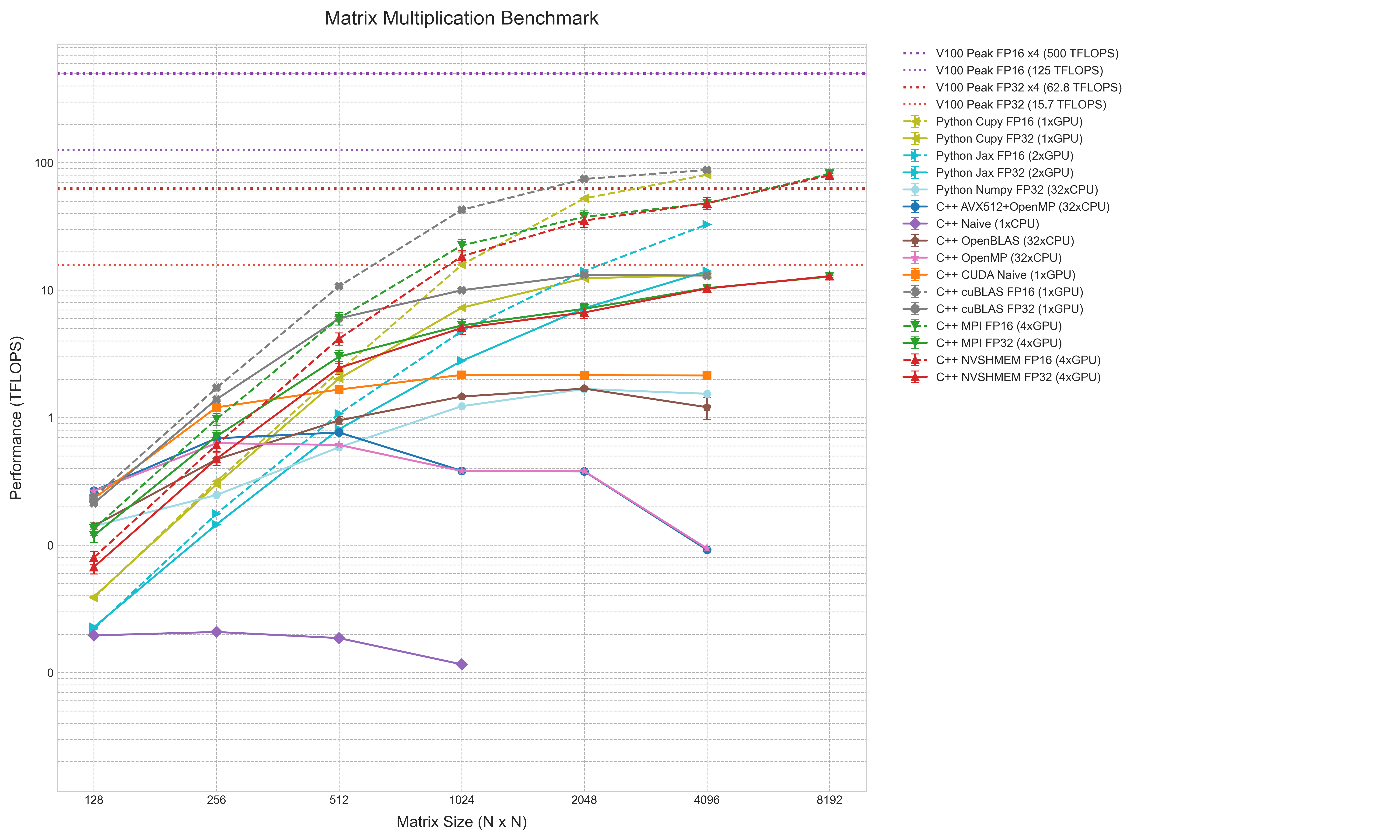
The performance results are summarized in a comprehensive chart, aggregating data from naive C++ loops to multi-GPU distributed computing using TFLOPS as a unified metric.
The chart uses log-log coordinates, with matrix size (N) on the horizontal axis and performance (TFLOPS) on the vertical axis. This clearly shows performance changes across several orders of magnitude. FP16 results are dashed lines, and error bars indicate 95% confidence intervals. Reference lines show theoretical peaks for V100 (FP32/FP16) and a 4-GPU system.
The hierarchy is clear: at the bottom is C++ Naive (1xCPU) at under 0.1 TFLOPS. Above it are multi-core CPU implementations (OpenMP, AVX512, NumPy) clustered between 1-2 TFLOPS. C++ OpenBLAS sits slightly higher.
GPU implementations occupy the upper regions. Even the C++ CUDA Naive kernel exceeds all CPU results, peaking over 2 TFLOPS. cuBLAS FP32 (C++ and CuPy) and 4-GPU MPI reach 10-15 TFLOPS, near the single-V100 FP32 peak. Python JAX FP32 (2xGPU) also resides here.
The top lines are FP16 implementations (cuBLAS, CuPy, MPI/NVSHMEM). These are significantly higher, with 4-GPU distributed computing reaching ~80 TFLOPS at , near the single-V100 FP16 peak. Python JAX FP16 (2xGPU) is notably lower than other FP16 implementations.
This chart synthesizes the performance gaps between simple implementations and hardware-optimized ones, reflecting the impact of compute platforms and precision choices on efficiency.
Would you like me to generate a detailed summary table comparing the peak TFLOPS achieved by each implementation for the largest matrix size tested?